
文章阅读:First Past the Post-Evaluating Query Optimization in MongoDB
这篇文章发表于ADC24,由悉尼大学的团队完成,同时也是2025年CMU-15799 Lecture#22的主讲论文
CMU提供的论文下载地址:https://15799.courses.cs.cmu.edu/spring2025/papers/23-mongodb/tao-adc2024.pdf
文章代码:https://github.com/michaelcahill/mongodb-fptp-paper
不知道大家怎么看,我觉得MongoDB一直是数据库产品中奇怪的一个东西,大佬们一直在炮轰这玩意性能不行……反正作为吃瓜位,我是没用过MongoDB的
不过既然Andy把这篇选上来了,那肯定应该有些值得说道的地方
Introduction
FPTP does not estimate costs for each execution plan, but rather partially executes the alternative plans in a round-robin race and observes the work done by each relative to the number of records returned.
替代计划与现有计划交叉运行,round-robin race? 有意思,后文说是速度提升了两倍,而且FPTP这一套方案并不用Cost-Based
Background and related work
简要介绍下Query Oprimzer的历史,这些内容在CMU15799里都能找到,这块对我而言没什么好看的。
另外还相对详细的介绍了MongoDB
The System R optimizer [3] restricted its attention to joins performed in a particular set of sequential patterns.
哦,这样吗?那改天看下System R是怎么做的?
MongoDB Query Model
At a low level, MongoDB stores data as BSON documents, which extends the JSON model to offer more data types and efficient encoding and decoding.
扩展的JSON?OK
Figure 1 provides an overview of the query processing workflow. We break down the whole process into three layers. In the network layer, MongoDB specifies a MongoDB Wire Protocol which is a simple socket-based, request-response-style protocol. Clients connect to the database following the protocol. In the executor layer, queries are received in the form of operation contexts. Some queries such as insert() do not require optimization. Therefore, these queries interact directly with the storage engine.

The winner of the race is then run to completion as the execution plan and is also cached for future queries with the same shape.
嗯哼,最终相同Shape的计划被缓存
这章配了一个很大的图,但却没有引用,似乎展示的是MongoDB Query Optimizer的流程

MongoDB’s FPTP Query Optimizer
A simplified explanation of FPTP is that the query optimizer initially executes all potential query plans in parallel and chooses the first one that completes a predefined amount of work. The winner of the race is then run to completion as the execution plan and is also cached for future queries with the same shape.
并行运行所有计划,然后将cost最小的那个缓存……啧,这个有点不太好评价,看看后面怎么说

一套Cost记录方案
关于各个Metric的详细解释
tieBreakers is a very small bonus number that is given when a plan contains no fetch operation (noFetchBonus), no blocking sort (noS ortBonus) or avoids index intersection (noI xisectBonus). eof Bonus is given if all possible documents are retrieved during the execution of the plan.
Evaluation Methodology
For each choice of selectivities, we identify which query plan is chosen by the optimizer, and plot that decision on a square diagram, where the x and y coordinates reflect the selectivities in that query. Each potential plan is indicated by a different color that can be assigned to the point.
将执行计划表示为图上的点,用颜色对计划进行区分(不同颜色表明计划所具有的选择性Selective)——我好奇的是,那这样岂不是产生几十几百个计划,然后进行比较?
Note:这里补充下关于选择性(Selective)的知识
选择性(Selectivity) 是谓词过滤数据的能力,常用来帮助优化器估算执行计划的代价。Selectivity = 通过某个条件过滤后保留的记录数 / 总记录数如果某个条件能筛选出很少的数据(如 age = 99),则选择性 低(值接近 0),意味着它是一个“有选择性的”条件。如果某个条件几乎不过滤数据(如 age > 0),则选择性 高(值接近 1),意味着它基本没有什么过滤能力。
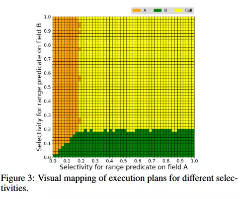
优化器在生成查询计划时,需要决定:先过滤还是先连接使用索引还是全表扫描选择什么样的连接算法(如嵌套循环、哈希连接)这些都依赖于谓词的选择性估算:低选择性(高过滤能力) → 适合尽早执行高选择性(低过滤能力) → 可能推迟执行或忽略索引We describe how a choice of plan is displayed in a plan diagram following [32]. For each query, the client will record eA, eB and PeA,eB (i.e. the execution plan for the query with selectivity eA and eB). The client will map PeA,eB to a position (i, j) on the grid. The magnitudes of i and j are proportional to eA and eB. Different execution plans are represented by pixels with different colors, as demonstrated in Figure 3 (which shows the optimal choice of plan from our first set of experiments)
下图的颜色标识如下:
IXSCAN_A: an index scan uses index A_1 on field A. This execution plan is represented by an orange pixel.
IXSCAN_B: an index scan uses index B_1 on field B. This execution plan is represented by a green pixel.
COLLSCAN: a collection scan (i.e. a table scan). This execution plan is represented by a yellow pixel.
The grid has dimension 50 × 50 and starts gray so that we can identify the abnormal behavior of the query optimizer (i.e. timeout or exceptions are thrown). When the experiment starts, the client keeps generating queries and trying to fill the grid with three colors, until all 502 positions on the grid have been visited. Algorithm 2 explains the entire visual mapping process.

一套用于绘图的算法……大伙们还是慢慢看吧😂
If the query optimizer has chosen the optimal plan, this ratio will be 1.0 and we represent this with white pixels. But the darker the color of a box, the worse the performance impact of the query optimizer’s (suboptimal) choice. An example of such a heat map visualizing the impact of FPTP performance is shown in Figure 4c.

emmm……所以,为什么有的计划好,有的计划差?
Evaluation of MongoDB’s FPTP Query Optimizer
Figure 4a plots the execution plans picked in this case by the MongoDB 7.0.1 query optimizer. We observe that both IXSCAN_A and IXSCAN_B are picked by the optimizer with equal chance, and as expected, the field where the query selectivity is lower (that is, fewer documents satisfy this predicate), has the index used.
4a边界在对角线上,说明Query Optimzer的性能是稳定的,所选的计划不会随查询的小扰动而变化
From Figures 5a and 5b we see that the collection scan is actually the best as long as more than about 20% of records satisfy the range predicate on B; however, even in these situations MongoDB chooses to use the available index on B; again, it never does a collection scan. Thus, the optimizer’s choice is even less accurate than in the previous scenario, with an overall accuracy of 19%
单Index的情况下,只有20%选择了IndexScan

Figure 6 shows the results of this third experiment. We again first visualize the query plans chosen by MongoDB’s FPTP optimizer (Figure 6a), the middle plot shows the optimal plan (Figure 6b), and the third plot is a visualization of the performance impact of MongoDB’s suboptimal plan choices (Figure 6c).
在使用覆盖引擎的情况下,情况又会发生变化——从图上来看的,Query Optimze的情况就没那么稳定
Overall, the experiments in this section demonstrate that while FPTP is a viable approach to query optimization with many good plan choices, it also suffers from what we call “preference bias” choosing index scans rather than full collections scans, even when the collection scan would perform much faster.
这一套方案会有“preference bias”导致无法达到最优,后面会对这个问题进行解释
Why does MongoDB’s FPTP Optimizer Avoid Collection Scans?
As we just saw in Section 4, MongoDB’s FPTP optimizer doesn’t choose collection scan plans, even for queries when it would run substantially faster than using an index.
哦哦
However, is this all there is to the issue? We modified the source code to produce a variant we call MongoDB+COLLSCAN that simply always adds a COLLSCAN plan to the set of candidate plans which MongoDB’s FPTP optimizer tries out
emmm……改源代码进行实验么,行吧
in Figures 8a–8c, We see that while the modified score is not a perfect adjustment, it makes the right decision in many of the queries, and the chosen plan is never much worse than the best possible.

问题是这个效果是人为修改的,实际能用不?

The scale of the workload evaluated here is considerably smaller than that common in real-world settings: we only measured cases where all indexes fit in memory.
啊这😅感觉不太妙
结语
图片排版不是很好😂时常找不到图
感觉没达到我想要效果,一方面我确实对文档数据库不了解,我对文档数据库的了解似乎与文章介绍的有些出入,这可能导致我没看懂文章
于我而言,自然是关心这套方案能不能用于传统的关系数据库上……但看完后,似乎并不能证明FPTP这套方案会优于传统的Cost-Base Estimation(而且机制介绍只有2.9一个小结,感觉没看够😂——还是只能写这么多?)
我想听听Andy怎么说(以及他为什么会选择这篇)——但目前为止(2025.5.3)Andy并还没更新上这节课的内容